Impedance Control Design for Single-Layer PCB Routing
Abstract
Impedance control is a critical aspect of high-speed PCB design, ensuring signal integrity by minimizing reflections and distortions. While multi-layer PCBs with dedicated ground planes are commonly used for impedance-controlled routing, single-layer PCBs also require careful impedance management in certain applications. This article explores the challenges and design techniques for achieving controlled impedance in single-layer PCBs, including trace geometry optimization, dielectric material selection, and reference plane considerations. Practical design guidelines and simulation approaches are discussed to help engineers implement effective single-layer impedance-controlled routing.
1. Introduction
Printed Circuit Boards (PCBs) are essential in modern electronics, supporting both analog and digital signal transmission. As signal frequencies increase, maintaining controlled impedance becomes crucial to prevent signal degradation due to reflections, crosstalk, and electromagnetic interference (EMI).
Multi-layer PCBs typically use microstrip or stripline configurations with dedicated ground planes for impedance control. However, single-layer PCBs—often used in cost-sensitive or space-constrained applications—pose unique challenges for impedance management due to the absence of an adjacent reference plane.
This paper examines the engineering considerations for single-layer PCB impedance control, including:
- Transmission line theory basics
- Impedance modeling for single-layer traces
- Design techniques to achieve target impedance
- Material and manufacturing impacts
- Simulation and validation methods
2. Transmission Line Basics
Impedance (Z₀) in a PCB trace is determined by its distributed inductance (L) and capacitance (C) per unit length:
[ Z_0 = \sqrt{\frac{L}{C}} ]
For a single-layer PCB, the primary impedance contributors are:
- Trace width (W) – Wider traces lower impedance.
- Trace thickness (T) – Thicker traces reduce impedance.
- Dielectric height (H) – Distance to the nearest reference (e.g., ground pour).
- Dielectric constant (εᵣ) – Affects capacitance.
Unlike microstrip lines (where a ground plane is directly beneath the signal trace), single-layer PCBs rely on coplanar waveguide or ground pour techniques for impedance control.

3. Impedance Modeling for Single-Layer PCBs
3.1 Coplanar Waveguide (CPW) Structure
A coplanar waveguide consists of a signal trace with adjacent ground conductors on the same layer. The impedance depends on:
[ Z_{0,CPW} \approx \frac{30\pi}{\sqrt{\epsilon_{eff}}} \cdot \frac{K(k’)}{K(k)} ]
Where:
- ( \epsilon_{eff} ) = Effective dielectric constant
- ( K(k) ) = Complete elliptic integral of the first kind
- ( k = \frac{W}{W + 2S} ) (W = trace width, S = gap to ground)
3.2 Single-Layer Microstrip with Ground Pour
If a ground pour exists on the same layer, the impedance can be approximated using modified microstrip equations:
[ Z_{0} \approx \frac{87}{\sqrt{\epsilon_r + 1.41}} \ln \left( \frac{5.98H}{0.8W + T} \right) ]
Where:
- ( H ) = Distance to the nearest reference (e.g., ground pour spacing)
- ( W ) = Trace width
- ( T ) = Trace thickness
3.3 Impact of No Ground Plane
Without a nearby ground reference, return current paths become unpredictable, leading to higher EMI and impedance variations. To mitigate this:
- Use a closely spaced ground pour around critical traces.
- Minimize discontinuities (e.g., sharp bends, vias).
- Avoid long ungrounded traces.
4. Design Techniques for Single-Layer Impedance Control
4.1 Trace Geometry Optimization
- Width Adjustment: Wider traces reduce impedance.
- Spacing to Ground: Tighter ground spacing increases capacitance, lowering impedance.
- Avoiding Sharp Corners: Use curved or 45° bends to minimize impedance discontinuities.
4.2 Ground Pour Strategies
- Coplanar Ground: Surround high-speed traces with ground copper to provide a return path.
- Stitching Vias: If a bottom ground exists, use vias to connect top-layer ground pours.
4.3 Dielectric Material Selection
- FR-4 (εᵣ ≈ 4.3): Common but has dispersion at high frequencies.
- Rogers Materials (εᵣ ≈ 2.2–10.2): Better high-frequency performance but costlier.
4.4 Manufacturing Tolerances
- Etching Variations: Account for ±10% impedance tolerance in fabrication.
- Copper Roughness: Affects high-frequency loss.
5. Simulation and Validation
5.1 Field Solver Tools
- ANSYS HFSS, Keysight ADS: Full-wave EM simulations for accurate modeling.
- Polar Si9000: Popular for impedance calculations.
5.2 Time-Domain Reflectometry (TDR)
- Measures actual impedance by sending a pulse and analyzing reflections.
5.3 Network Analyzer Measurements
- Validates impedance and insertion loss in fabricated boards.
6. Practical Design Example
Target: 50Ω impedance on a 1.6mm FR-4 single-layer PCB.
Approach:
- Use a 2.5mm trace width with 0.5mm spacing to ground pour.
- Simulate in Polar Si9000, adjusting for manufacturing tolerances.
- Verify with TDR after fabrication.
7. Conclusion
Single-layer PCB impedance control is challenging but achievable with careful design. Key strategies include optimizing trace geometry, using coplanar ground structures, and validating with simulation and testing. While multi-layer PCBs are preferred for high-speed designs, single-layer impedance techniques remain valuable for cost-sensitive applications.